Bank Marketing Data Set Classification

The aim of this projects is to explain how machine learning can help in a bank marketing campaign.The goal of our classifier is to predict using the logistic regression algorithm if a client may subscribe to a fixed term deposit. Often, more than one contact to the same client was required, in order to access if the product (bank term deposit) would be (‘yes’) or not (‘no’) subscribed.

Data Set Information: source https://archive.ics.uci.edu/ml/datasets/Bank+Marketing

The data is related with direct marketing campaigns of a Portuguese banking institution. The marketing campaigns were based on phone calls. Often, more than one contact to the same client was required, in order to access if the product (bank term deposit) would be (‘yes’) or not (‘no’) subscribed.

There are four datasets: 1) bank-additional-full.csv with all examples (41188) and 20 inputs, ordered by date (from May 2008 to November 2010), very close to the data analyzed in [Moro et al., 2014] 2) bank-additional.csv with 10% of the examples (4119), randomly selected from 1), and 20 inputs. 3) bank-full.csv with all examples and 17 inputs, ordered by date (older version of this dataset with less inputs). 4) bank.csv with 10% of the examples and 17 inputs, randomly selected from 3 (older version of this dataset with less inputs). The smallest datasets are provided to test more computationally demanding machine learning algorithms (e.g., SVM).

The classification goal is to predict if the client will subscribe (yes/no) a term deposit (variable y).

Attribute Information:

Input variables: #bank client data: 1 - age (numeric) 2 - job : type of job (categorical: ‘admin.’,’blue-collar’,’entrepreneur’,’housemaid’,’management’,’retired’,’self-employed’,’services’,’student’,’technician’,’unemployed’,’unknown’) 3 - marital : marital status (categorical: ‘divorced’,’married’,’single’,’unknown’; note: ‘divorced’ means divorced or widowed) 4 - education (categorical: ‘basic.4y’,’basic.6y’,’basic.9y’,’high.school’,’illiterate’,’professional.course’,’university.degree’,’unknown’) 5 - default: has credit in default? (categorical: ‘no’,’yes’,’unknown’) 6 - housing: has housing loan? (categorical: ‘no’,’yes’,’unknown’) 7 - loan: has personal loan? (categorical: ‘no’,’yes’,’unknown’) #related with the last contact of the current campaign: 8 - contact: contact communication type (categorical: ‘cellular’,’telephone’) 9 - month: last contact month of year (categorical: ‘jan’, ‘feb’, ‘mar’, …, ‘nov’, ‘dec’) 10 - day_of_week: last contact day of the week (categorical: ‘mon’,’tue’,’wed’,’thu’,’fri’) 11 - duration: last contact duration, in seconds (numeric). Important note: this attribute highly affects the output target (e.g., if duration=0 then y=’no’). Yet, the duration is not known before a call is performed. Also, after the end of the call y is obviously known. Thus, this input should only be included for benchmark purposes and should be discarded if the intention is to have a realistic predictive model. #other attributes: 12 - campaign: number of contacts performed during this campaign and for this client (numeric, includes last contact) 13 - pdays: number of days that passed by after the client was last contacted from a previous campaign (numeric; 999 means client was not previously contacted) 14 - previous: number of contacts performed before this campaign and for this client (numeric) 15 - poutcome: outcome of the previous marketing campaign (categorical: ‘failure’,’nonexistent’,’success’) #social and economic context attributes 16 - emp.var.rate: employment variation rate - quarterly indicator (numeric) 17 - cons.price.idx: consumer price index - monthly indicator (numeric) 18 - cons.conf.idx: consumer confidence index - monthly indicator (numeric) 19 - euribor3m: euribor 3 month rate - daily indicator (numeric) 20 - nr.employed: number of employees - quarterly indicator (numeric)

Output variable (desired target): 21 - y - has the client subscribed a term deposit? (binary: ‘yes’,’no’)

Load Dataset

import pandas as pd
import numpy as np

df = pd.read_csv('./bank/bank.csv', sep=';')

print ('Data read into a pandas dataframe!')

Data read into a pandas dataframe!

df.head()

	age	job	marital	education	default	balance	housing	loan	contact	day	month	duration	campaign	pdays	previous	poutcome	y
0	30	unemployed	married	primary	no	1787	no	no	cellular	19	oct	79	1	-1	0	unknown	no
1	33	services	married	secondary	no	4789	yes	yes	cellular	11	may	220	1	339	4	failure	no
2	35	management	single	tertiary	no	1350	yes	no	cellular	16	apr	185	1	330	1	failure	no
3	30	management	married	tertiary	no	1476	yes	yes	unknown	3	jun	199	4	-1	0	unknown	no
4	59	blue-collar	married	secondary	no	0	yes	no	unknown	5	may	226	1	-1	0	unknown	no

df.tail()

	age	job	marital	education	default	balance	housing	loan	contact	day	month	duration	campaign	pdays	previous	poutcome	y
4516	33	services	married	secondary	no	-333	yes	no	cellular	30	jul	329	5	-1	0	unknown	no
4517	57	self-employed	married	tertiary	yes	-3313	yes	yes	unknown	9	may	153	1	-1	0	unknown	no
4518	57	technician	married	secondary	no	295	no	no	cellular	19	aug	151	11	-1	0	unknown	no
4519	28	blue-collar	married	secondary	no	1137	no	no	cellular	6	feb	129	4	211	3	other	no
4520	44	entrepreneur	single	tertiary	no	1136	yes	yes	cellular	3	apr	345	2	249	7	other	no

df.shape

(4521, 17)

df.info()

<class 'pandas.core.frame.DataFrame'>
RangeIndex: 4521 entries, 0 to 4520
Data columns (total 17 columns):
 #   Column     Non-Null Count  Dtype 
---  ------     --------------  ----- 
 0   age        4521 non-null   int64 
 1   job        4521 non-null   object
 2   marital    4521 non-null   object
 3   education  4521 non-null   object
 4   default    4521 non-null   object
 5   balance    4521 non-null   int64 
 6   housing    4521 non-null   object
 7   loan       4521 non-null   object
 8   contact    4521 non-null   object
 9   day        4521 non-null   int64 
 10  month      4521 non-null   object
 11  duration   4521 non-null   int64 
 12  campaign   4521 non-null   int64 
 13  pdays      4521 non-null   int64 
 14  previous   4521 non-null   int64 
 15  poutcome   4521 non-null   object
 16  y          4521 non-null   object
dtypes: int64(7), object(10)
memory usage: 600.6+ KB

df.describe().T

	count	mean	std	min	25%	50%	75%	max
age	4521.0	41.170095	10.576211	19.0	33.0	39.0	49.0	87.0
balance	4521.0	1422.657819	3009.638142	-3313.0	69.0	444.0	1480.0	71188.0
day	4521.0	15.915284	8.247667	1.0	9.0	16.0	21.0	31.0
duration	4521.0	263.961292	259.856633	4.0	104.0	185.0	329.0	3025.0
campaign	4521.0	2.793630	3.109807	1.0	1.0	2.0	3.0	50.0
pdays	4521.0	39.766645	100.121124	-1.0	-1.0	-1.0	-1.0	871.0
previous	4521.0	0.542579	1.693562	0.0	0.0	0.0	0.0	25.0

print("Train Data:")
print(df.isnull().sum(), "\n")

Train Data:
age          0
job          0
marital      0
education    0
default      0
balance      0
housing      0
loan         0
contact      0
day          0
month        0
duration     0
campaign     0
pdays        0
previous     0
poutcome     0
y            0
dtype: int64 

replace y column value

df['y'] = df.y.replace({"yes": 1, "no": 0})

# iterated through df and stored data with datatype as 'object' to new variable cat_col
cat_col = [n for n in df.columns if df[n].dtypes == 'object']

df.head()

	age	job	marital	education	default	balance	housing	loan	contact	day	month	duration	campaign	pdays	previous	poutcome	y
0	30	unemployed	married	primary	no	1787	no	no	cellular	19	oct	79	1	-1	0	unknown	0
1	33	services	married	secondary	no	4789	yes	yes	cellular	11	may	220	1	339	4	failure	0
2	35	management	single	tertiary	no	1350	yes	no	cellular	16	apr	185	1	330	1	failure	0
3	30	management	married	tertiary	no	1476	yes	yes	unknown	3	jun	199	4	-1	0	unknown	0
4	59	blue-collar	married	secondary	no	0	yes	no	unknown	5	may	226	1	-1	0	unknown	0

analysis on our dependent variable ‘y’ to check for data imbalance

%matplotlib inline 

import matplotlib as mpl
import matplotlib.pyplot as plt
all_row = len(df)
no_sub = len(df[df['y'] == 0])
sub = len(df[df['y']==1])
percentage_no_sub = (no_sub/all_row) * 100
percentage_sub = (sub/all_row) * 100

print('% no subcription: ', percentage_no_sub)
print('% subcription: ', percentage_sub)
my_color = 'rg'
df['y'].value_counts().plot(kind='bar')

% no subcription:  88.47600088476001
% subcription:  11.523999115239992





<matplotlib.axes._subplots.AxesSubplot at 0x7fed81617970>

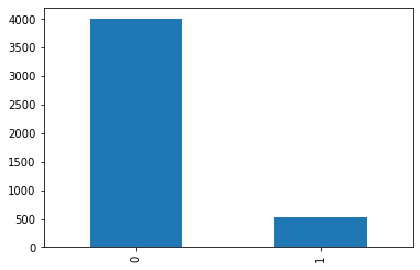
from analysis above, we can see majority data is no subcription 88%, dependent variable is no_sub

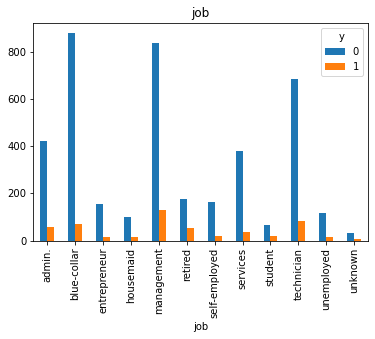
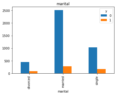
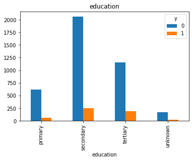
Visualisation

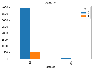
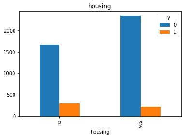
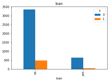
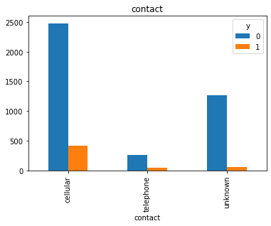
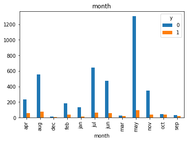
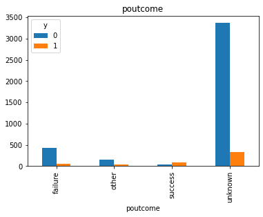
#Visualization from our categorical datas top see if we can get insigts from there
for col in cat_col:
    pd.crosstab(df[col], df.y).plot(kind = 'bar')
    plt.title(col)

df['pdays'].value_counts()

-1      3705
 182      23
 183      20
 363      12
 92       12
        ... 
 222       1
 210       1
 206       1
 162       1
 28        1
Name: pdays, Length: 292, dtype: int64

df['contact'].value_counts()

cellular     2896
unknown      1324
telephone     301
Name: contact, dtype: int64

# replace contact with value
df['contact'] = df.contact.replace({"cellular": 1, "unknown": 0,"telephone":2})

df = pd.get_dummies(df,columns=['job','marital','education','default','housing','loan','month','poutcome'],drop_first = True)

df.head()

	age	balance	contact	day	duration	campaign	pdays	previous	y	job_blue-collar	...	month_jul	month_jun	month_mar	month_may	month_nov	month_oct	month_sep	poutcome_other	poutcome_success	poutcome_unknown
0	30	1787	1	19	79	1	-1	0	0	0	...	0	0	0	0	0	1	0	0	0	1
1	33	4789	1	11	220	1	339	4	0	0	...	0	0	0	1	0	0	0	0	0	0
2	35	1350	1	16	185	1	330	1	0	0	...	0	0	0	0	0	0	0	0	0	0
3	30	1476	0	3	199	4	-1	0	0	0	...	0	1	0	0	0	0	0	0	0	1
4	59	0	0	5	226	1	-1	0	0	1	...	0	0	0	1	0	0	0	0	0	1

5 rows × 42 columns

df.shape

(4521, 42)

from sklearn.model_selection import train_test_split
X=df.loc[:,df.columns != 'y']
y=df.loc[:,df.columns == 'y']
x_train, x_cv, y_train, y_cv = train_test_split(X, y, test_size=0.2)
print('x train ',len(x_train))
print('x test ',len(x_cv))
print('y train ',len(y_train))
print('y test ',len(y_cv))

x train  3616
x test  905
y train  3616
y test  905

LOGISTIC REGRESSION

#(a)LOGISTIC REGRESSION

from sklearn.linear_model import LogisticRegression

model=LogisticRegression()

model.fit(x_train,y_train)

/Users/mac/.pyenv/versions/anaconda3-2020.07/lib/python3.8/site-packages/sklearn/utils/validation.py:63: DataConversionWarning: A column-vector y was passed when a 1d array was expected. Please change the shape of y to (n_samples, ), for example using ravel().
  return f(*args, **kwargs)
/Users/mac/.pyenv/versions/anaconda3-2020.07/lib/python3.8/site-packages/sklearn/linear_model/_logistic.py:763: ConvergenceWarning: lbfgs failed to converge (status=1):
STOP: TOTAL NO. of ITERATIONS REACHED LIMIT.

Increase the number of iterations (max_iter) or scale the data as shown in:
    https://scikit-learn.org/stable/modules/preprocessing.html
Please also refer to the documentation for alternative solver options:
    https://scikit-learn.org/stable/modules/linear_model.html#logistic-regression
  n_iter_i = _check_optimize_result(





LogisticRegression()

pred_cv=model.predict(x_cv)

from sklearn.metrics import accuracy_score
from sklearn.metrics import confusion_matrix

print(accuracy_score(y_cv,pred_cv))
matrix=confusion_matrix(y_cv,pred_cv)
print(matrix)

0.9005524861878453
[[793   7]
 [ 83  22]]

K-NEAREST NEIGHBOR(kNN) ALGORITHM

#(f)K-NEAREST NEIGHBOR(kNN) ALGORITHM

from sklearn.neighbors import KNeighborsClassifier
kNN=KNeighborsClassifier()
kNN.fit(x_train,y_train)

pred_cv5=kNN.predict(x_cv)

print(accuracy_score(y_cv,pred_cv5))
matrix5=confusion_matrix(y_cv,pred_cv5)
print(matrix5)

/Users/mac/.pyenv/versions/anaconda3-2020.07/lib/python3.8/site-packages/sklearn/neighbors/_classification.py:179: DataConversionWarning: A column-vector y was passed when a 1d array was expected. Please change the shape of y to (n_samples,), for example using ravel().
  return self._fit(X, y)


0.8784530386740331
[[777  23]
 [ 87  18]]

SUPPORT VECTOR MACHINE (SVM) ALGORITHM

from sklearn import svm
svm_model=svm.SVC()
svm_model.fit(x_train,y_train)
pred_cv3=svm_model.predict(x_cv)
print(accuracy_score(y_cv,pred_cv3))
matrix3=confusion_matrix(y_cv,pred_cv3)
print(matrix3)

/Users/mac/.pyenv/versions/anaconda3-2020.07/lib/python3.8/site-packages/sklearn/utils/validation.py:63: DataConversionWarning: A column-vector y was passed when a 1d array was expected. Please change the shape of y to (n_samples, ), for example using ravel().
  return f(*args, **kwargs)


0.8839779005524862
[[800   0]
 [105   0]]

DECISION TREE ALGORITHM

from sklearn import tree
dt=tree.DecisionTreeClassifier()
dt.fit(x_train,y_train)
pred_cv1=dt.predict(x_cv)
print(accuracy_score(y_cv,pred_cv1))
matrix1=confusion_matrix(y_cv,pred_cv1)
print(matrix1)

0.8895027624309392
[[750  50]
 [ 50  55]]

RANDOM FOREST ALGORITHM

from sklearn.ensemble import RandomForestClassifier
rf=RandomForestClassifier()
rf.fit(x_train,y_train)
pred_cv2=rf.predict(x_cv)
print(accuracy_score(y_cv,pred_cv2))
matrix2=confusion_matrix(y_cv,pred_cv2)
print(matrix2)

<ipython-input-80-d123f799bf67>:3: DataConversionWarning: A column-vector y was passed when a 1d array was expected. Please change the shape of y to (n_samples,), for example using ravel().
  rf.fit(x_train,y_train)


0.8983425414364641
[[791   9]
 [ 83  22]]

NAIVE BAYES ALGORITHM

from sklearn.naive_bayes import GaussianNB 
nb=GaussianNB()
nb.fit(x_train,y_train)

pred_cv4=nb.predict(x_cv)

print(accuracy_score(y_cv,pred_cv4))
matrix4=confusion_matrix(y_cv,pred_cv4)
print(matrix4)

0.8640883977900552
[[725  75]
 [ 48  57]]


/Users/mac/.pyenv/versions/anaconda3-2020.07/lib/python3.8/site-packages/sklearn/utils/validation.py:63: DataConversionWarning: A column-vector y was passed when a 1d array was expected. Please change the shape of y to (n_samples, ), for example using ravel().
  return f(*args, **kwargs)

print("Logistic Regression:", accuracy_score(y_cv,pred_cv))
print("Decision Tree:", accuracy_score(y_cv,pred_cv1))
print("Random Forest:", accuracy_score(y_cv,pred_cv2))
print("SVM:", accuracy_score(y_cv,pred_cv3))
print("Naive Bayes:", accuracy_score(y_cv,pred_cv4))
print("KNN:", accuracy_score(y_cv,pred_cv5))

Logistic Regression: 0.9005524861878453
Decision Tree: 0.8895027624309392
Random Forest: 0.8983425414364641
SVM: 0.8839779005524862
Naive Bayes: 0.8640883977900552
KNN: 0.8784530386740331