Analysis NYC Property Sales
NYC Property Sales Introduction
The aim of this projects is to introduce you to practical statistic with Python as concrete and as consistent as possible. Using what you’ve learned; download the NYC Property Sales Dataset from Kaggle. This dataset is a record of every building or building unit (apartment, etc.) sold in the New York City property market over a 12-month period.
This dataset contains the location, address, type, sale price, and sale date of building units sold. A reference on the trickier fields:
BOROUGH: A digit code for the borough the property is located in; in order these are Manhattan (1), Bronx (2), Brooklyn (3), Queens (4), and Staten Island (5).BLOCK;LOT: The combination of borough, block, and lot forms a unique key for property in New York City. Commonly called a BBL.BUILDING CLASS AT PRESENTandBUILDING CLASS AT TIME OF SALE: The type of building at various points in time.
Note that because this is a financial transaction dataset, there are some points that need to be kept in mind:
- Many sales occur with a nonsensically small dollar amount: $0 most commonly. These sales are actually transfers of deeds between parties: for example, parents transferring ownership to their home to a child after moving out for retirement.
- This dataset uses the financial definition of a building/building unit, for tax purposes. In case a single entity owns the building in question, a sale covers the value of the entire building. In case a building is owned piecemeal by its residents (a condominium), a sale refers to a single apartment (or group of apartments) owned by some individual.
Formulate a question and derive a statistical hypothesis test to answer the question. You have to demonstrate that you’re able to make decisions using data in a scientific manner. Examples of questions can be:
- Is there a difference in unit sold between property built in 1900-2000 and 2001 so on?
- Is there a difference in unit sold based on building category?
- What can you discover about New York City real estate by looking at a year’s worth of raw transaction records? Can you spot trends in the market?
Please make sure that you have completed the lesson for this course, namely Python and Practical Statistics which is part of this Program.
Note: You can take a look at Project Rubric below:
| Code Review | |
|---|---|
| CRITERIA | SPECIFICATIONS |
| Mean | Student implement mean to specifics column/data using pandas, numpy, or scipy |
| Median | Student implement median to specifics column/data using pandas, numpy, or scipy |
| Modus | Student implement modus to specifics column/data using pandas, numpy, or scipy |
| Central Tendencies | Implementing Central Tendencies through dataset |
| Box Plot | Implementing Box Plot to visualize spesific data |
| Z-Score | Implementing Z-score concept to specific data |
| Probability Distribution | Student analyzing distribution of data and gain insight from the distribution |
| Intervals | Implementing Confidence or Prediction Intervals |
| Hypotesis Testing | Made 1 Hypotesis and get conclusion from data |
| Preprocessing | Student preprocess dataset before applying the statistical treatment. |
| Does the code run without errors? | The code runs without errors. All code is functional and formatted properly. |
| Readability | |
|---|---|
| CRITERIA | SPECIFICATIONS |
| Well Documented | All cell in notebook are well documented with markdown above each cell explaining the code |
| Analysis | |
|---|---|
| CRITERIA | SPECIFICATIONS |
| Overall Analysis | Gain an insight/conclusion of overall plots that answer the hypotesis |
Focus on “Graded-Function” sections.
Data Preparation
Load the library you need.
Get your NYC property data from here and load the dataframe to your notebook.
# Get your import statement here
import pandas as pd
import numpy as np
# Load your dataset here
df = pd.read_csv('nyc-rolling-sales.csv')

print ('Data read into a pandas dataframe!')
Data read into a pandas dataframe!
Let’s view the top 5 rows of the dataset using the head() function.
# Write your syntax here
df.head()
| Unnamed: 0 | BOROUGH | NEIGHBORHOOD | BUILDING CLASS CATEGORY | TAX CLASS AT PRESENT | BLOCK | LOT | EASE-MENT | BUILDING CLASS AT PRESENT | ADDRESS | ... | RESIDENTIAL UNITS | COMMERCIAL UNITS | TOTAL UNITS | LAND SQUARE FEET | GROSS SQUARE FEET | YEAR BUILT | TAX CLASS AT TIME OF SALE | BUILDING CLASS AT TIME OF SALE | SALE PRICE | SALE DATE | |
|---|---|---|---|---|---|---|---|---|---|---|---|---|---|---|---|---|---|---|---|---|---|
| 0 | 4 | 1 | ALPHABET CITY | 07 RENTALS - WALKUP APARTMENTS | 2A | 392 | 6 | C2 | 153 AVENUE B | ... | 5 | 0 | 5 | 1633 | 6440 | 1900 | 2 | C2 | 6625000 | 2017-07-19 00:00:00 | |
| 1 | 5 | 1 | ALPHABET CITY | 07 RENTALS - WALKUP APARTMENTS | 2 | 399 | 26 | C7 | 234 EAST 4TH STREET | ... | 28 | 3 | 31 | 4616 | 18690 | 1900 | 2 | C7 | - | 2016-12-14 00:00:00 | |
| 2 | 6 | 1 | ALPHABET CITY | 07 RENTALS - WALKUP APARTMENTS | 2 | 399 | 39 | C7 | 197 EAST 3RD STREET | ... | 16 | 1 | 17 | 2212 | 7803 | 1900 | 2 | C7 | - | 2016-12-09 00:00:00 | |
| 3 | 7 | 1 | ALPHABET CITY | 07 RENTALS - WALKUP APARTMENTS | 2B | 402 | 21 | C4 | 154 EAST 7TH STREET | ... | 10 | 0 | 10 | 2272 | 6794 | 1913 | 2 | C4 | 3936272 | 2016-09-23 00:00:00 | |
| 4 | 8 | 1 | ALPHABET CITY | 07 RENTALS - WALKUP APARTMENTS | 2A | 404 | 55 | C2 | 301 EAST 10TH STREET | ... | 6 | 0 | 6 | 2369 | 4615 | 1900 | 2 | C2 | 8000000 | 2016-11-17 00:00:00 |
5 rows × 22 columns
We can also veiw the bottom 5 rows of the dataset using the tail() function.
# Write your syntax here
df.tail()
| Unnamed: 0 | BOROUGH | NEIGHBORHOOD | BUILDING CLASS CATEGORY | TAX CLASS AT PRESENT | BLOCK | LOT | EASE-MENT | BUILDING CLASS AT PRESENT | ADDRESS | ... | RESIDENTIAL UNITS | COMMERCIAL UNITS | TOTAL UNITS | LAND SQUARE FEET | GROSS SQUARE FEET | YEAR BUILT | TAX CLASS AT TIME OF SALE | BUILDING CLASS AT TIME OF SALE | SALE PRICE | SALE DATE | |
|---|---|---|---|---|---|---|---|---|---|---|---|---|---|---|---|---|---|---|---|---|---|
| 84543 | 8409 | 5 | WOODROW | 02 TWO FAMILY DWELLINGS | 1 | 7349 | 34 | B9 | 37 QUAIL LANE | ... | 2 | 0 | 2 | 2400 | 2575 | 1998 | 1 | B9 | 450000 | 2016-11-28 00:00:00 | |
| 84544 | 8410 | 5 | WOODROW | 02 TWO FAMILY DWELLINGS | 1 | 7349 | 78 | B9 | 32 PHEASANT LANE | ... | 2 | 0 | 2 | 2498 | 2377 | 1998 | 1 | B9 | 550000 | 2017-04-21 00:00:00 | |
| 84545 | 8411 | 5 | WOODROW | 02 TWO FAMILY DWELLINGS | 1 | 7351 | 60 | B2 | 49 PITNEY AVENUE | ... | 2 | 0 | 2 | 4000 | 1496 | 1925 | 1 | B2 | 460000 | 2017-07-05 00:00:00 | |
| 84546 | 8412 | 5 | WOODROW | 22 STORE BUILDINGS | 4 | 7100 | 28 | K6 | 2730 ARTHUR KILL ROAD | ... | 0 | 7 | 7 | 208033 | 64117 | 2001 | 4 | K6 | 11693337 | 2016-12-21 00:00:00 | |
| 84547 | 8413 | 5 | WOODROW | 35 INDOOR PUBLIC AND CULTURAL FACILITIES | 4 | 7105 | 679 | P9 | 155 CLAY PIT ROAD | ... | 0 | 1 | 1 | 10796 | 2400 | 2006 | 4 | P9 | 69300 | 2016-10-27 00:00:00 |
5 rows × 22 columns
BOROUGH: A digit code for the borough the property is located in; in order these are Manhattan (1), Bronx (2), Brooklyn (3), Queens (4), and Staten Island (5).
To view the dimensions of the dataframe, we use the .shape parameter. Expected result: (84548, 22)
# Write your syntax here
df.shape
(84548, 22)
According to this official page, Ease-ment is “is a right, such as a right of way, which allows an entity to make limited use of another’s real property. For example: MTA railroad tracks that run across a portion of another property”. Also, the Unnamed column is not mentioned and was likely used for iterating through records. So, those two columns are removed for now.
# Drop 'Unnamed: 0' and 'EASE-MENT' features using .drop function
df.drop(['Unnamed: 0','EASE-MENT'], axis=1, inplace=True)
df.head()
| BOROUGH | NEIGHBORHOOD | BUILDING CLASS CATEGORY | TAX CLASS AT PRESENT | BLOCK | LOT | BUILDING CLASS AT PRESENT | ADDRESS | APARTMENT NUMBER | ZIP CODE | RESIDENTIAL UNITS | COMMERCIAL UNITS | TOTAL UNITS | LAND SQUARE FEET | GROSS SQUARE FEET | YEAR BUILT | TAX CLASS AT TIME OF SALE | BUILDING CLASS AT TIME OF SALE | SALE PRICE | SALE DATE | |
|---|---|---|---|---|---|---|---|---|---|---|---|---|---|---|---|---|---|---|---|---|
| 0 | 1 | ALPHABET CITY | 07 RENTALS - WALKUP APARTMENTS | 2A | 392 | 6 | C2 | 153 AVENUE B | 10009 | 5 | 0 | 5 | 1633 | 6440 | 1900 | 2 | C2 | 6625000 | 2017-07-19 00:00:00 | |
| 1 | 1 | ALPHABET CITY | 07 RENTALS - WALKUP APARTMENTS | 2 | 399 | 26 | C7 | 234 EAST 4TH STREET | 10009 | 28 | 3 | 31 | 4616 | 18690 | 1900 | 2 | C7 | - | 2016-12-14 00:00:00 | |
| 2 | 1 | ALPHABET CITY | 07 RENTALS - WALKUP APARTMENTS | 2 | 399 | 39 | C7 | 197 EAST 3RD STREET | 10009 | 16 | 1 | 17 | 2212 | 7803 | 1900 | 2 | C7 | - | 2016-12-09 00:00:00 | |
| 3 | 1 | ALPHABET CITY | 07 RENTALS - WALKUP APARTMENTS | 2B | 402 | 21 | C4 | 154 EAST 7TH STREET | 10009 | 10 | 0 | 10 | 2272 | 6794 | 1913 | 2 | C4 | 3936272 | 2016-09-23 00:00:00 | |
| 4 | 1 | ALPHABET CITY | 07 RENTALS - WALKUP APARTMENTS | 2A | 404 | 55 | C2 | 301 EAST 10TH STREET | 10009 | 6 | 0 | 6 | 2369 | 4615 | 1900 | 2 | C2 | 8000000 | 2016-11-17 00:00:00 |
Let’s view Dtype of each features in dataframe using .info() function.
df.info()
<class 'pandas.core.frame.DataFrame'>
RangeIndex: 84548 entries, 0 to 84547
Data columns (total 20 columns):
 #   Column                          Non-Null Count  Dtype
---  ------                          --------------  -----
 0   BOROUGH                         84548 non-null  int64
 1   NEIGHBORHOOD                    84548 non-null  object
 2   BUILDING CLASS CATEGORY         84548 non-null  object
 3   TAX CLASS AT PRESENT            84548 non-null  object
 4   BLOCK                           84548 non-null  int64
 5   LOT                             84548 non-null  int64
 6   BUILDING CLASS AT PRESENT       84548 non-null  object
 7   ADDRESS                         84548 non-null  object
 8   APARTMENT NUMBER                84548 non-null  object
 9   ZIP CODE                        84548 non-null  int64
 10  RESIDENTIAL UNITS               84548 non-null  int64
 11  COMMERCIAL UNITS                84548 non-null  int64
 12  TOTAL UNITS                     84548 non-null  int64
 13  LAND SQUARE FEET                84548 non-null  object
 14  GROSS SQUARE FEET               84548 non-null  object
 15  YEAR BUILT                      84548 non-null  int64
 16  TAX CLASS AT TIME OF SALE       84548 non-null  int64
 17  BUILDING CLASS AT TIME OF SALE  84548 non-null  object
 18  SALE PRICE                      84548 non-null  object
 19  SALE DATE                       84548 non-null  object
dtypes: int64(9), object(11)
memory usage: 12.9+ MB
It looks like empty records are not being treated as NA. We convert columns to their appropriate data types to obtain NAs.
#First, let's check which columns should be categorical
print('Column name')
for col in df.columns:
    if df[col].dtype=='object':
        print(col, df[col].nunique())
Column name
NEIGHBORHOOD 254
BUILDING CLASS CATEGORY 47
TAX CLASS AT PRESENT 11
BUILDING CLASS AT PRESENT 167
ADDRESS 67563
APARTMENT NUMBER 3989
LAND SQUARE FEET 6062
GROSS SQUARE FEET 5691
BUILDING CLASS AT TIME OF SALE 166
SALE PRICE 10008
SALE DATE 364
# LAND SQUARE FEET,GROSS SQUARE FEET, SALE PRICE, BOROUGH should be numeric.
# SALE DATE datetime format.
# categorical: NEIGHBORHOOD, BUILDING CLASS CATEGORY, TAX CLASS AT PRESENT, BUILDING CLASS AT PRESENT,
# BUILDING CLASS AT TIME OF SALE, TAX CLASS AT TIME OF SALE,BOROUGH

numer = ['LAND SQUARE FEET','GROSS SQUARE FEET', 'SALE PRICE', 'BOROUGH']
for col in numer: # coerce for missing values
    df[col] = pd.to_numeric(df[col], errors='coerce')

categ = ['NEIGHBORHOOD', 'BUILDING CLASS CATEGORY', 'TAX CLASS AT PRESENT', 'BUILDING CLASS AT PRESENT', 'BUILDING CLASS AT TIME OF SALE', 'TAX CLASS AT TIME OF SALE']
for col in categ:
    df[col] = df[col].astype('category')

df['SALE DATE'] = pd.to_datetime(df['SALE DATE'], errors='coerce')
Our dataset is ready for checking missing values.
missing = df.isnull().sum()/len(df)*100

print(pd.DataFrame([missing[missing>0],pd.Series(df.isnull().sum()[df.isnull().sum()>1000])], index=['percent missing','how many missing']))
                  LAND SQUARE FEET  GROSS SQUARE FEET   SALE PRICE
percent missing          31.049818          32.658372     17.22217
how many missing      26252.000000       27612.000000  14561.00000
Around 30% of GROSS SF and LAND SF are missing. Furthermore, around 17% of SALE PRICE is also missing.
We can fill in the missing value from one column to another, which will help us reduce missing values. Expected values:
(6, 20)
(1366, 20)
print(df[(df['LAND SQUARE FEET'].isnull()) & (df['GROSS SQUARE FEET'].notnull())].shape)
print(df[(df['LAND SQUARE FEET'].notnull()) & (df['GROSS SQUARE FEET'].isnull())].shape)
(6, 20)
(1366, 20)
There are 1372 rows that can be filled in with their approximate values.
df['LAND SQUARE FEET'] = df['LAND SQUARE FEET'].mask((df['LAND SQUARE FEET'].isnull()) & (df['GROSS SQUARE FEET'].notnull()), df['GROSS SQUARE FEET'])
df['GROSS SQUARE FEET'] = df['GROSS SQUARE FEET'].mask((df['LAND SQUARE FEET'].notnull()) & (df['GROSS SQUARE FEET'].isnull()), df['LAND SQUARE FEET'])
#  Check for duplicates before

print(sum(df.duplicated()))

df[df.duplicated(keep=False)].sort_values(['NEIGHBORHOOD', 'ADDRESS']).head(10)

# df.duplicated() automatically excludes duplicates, to keep duplicates in df we use keep=False

# in df.duplicated(df.columns) we can specify column names to look for duplicates only in those mentioned columns.
765
| BOROUGH | NEIGHBORHOOD | BUILDING CLASS CATEGORY | TAX CLASS AT PRESENT | BLOCK | LOT | BUILDING CLASS AT PRESENT | ADDRESS | APARTMENT NUMBER | ZIP CODE | RESIDENTIAL UNITS | COMMERCIAL UNITS | TOTAL UNITS | LAND SQUARE FEET | GROSS SQUARE FEET | YEAR BUILT | TAX CLASS AT TIME OF SALE | BUILDING CLASS AT TIME OF SALE | SALE PRICE | SALE DATE | |
|---|---|---|---|---|---|---|---|---|---|---|---|---|---|---|---|---|---|---|---|---|
| 76286 | 5 | ANNADALE | 02 TWO FAMILY DWELLINGS | 1 | 6350 | 7 | B2 | 106 BENNETT PLACE | 10312 | 2 | 0 | 2 | 8000.0 | 4208.0 | 1985 | 1 | B2 | NaN | 2017-06-27 | |
| 76287 | 5 | ANNADALE | 02 TWO FAMILY DWELLINGS | 1 | 6350 | 7 | B2 | 106 BENNETT PLACE | 10312 | 2 | 0 | 2 | 8000.0 | 4208.0 | 1985 | 1 | B2 | NaN | 2017-06-27 | |
| 76322 | 5 | ANNADALE | 05 TAX CLASS 1 VACANT LAND | 1B | 6459 | 28 | V0 | N/A HYLAN BOULEVARD | 0 | 0 | 0 | 0 | 6667.0 | 6667.0 | 0 | 1 | V0 | NaN | 2017-05-11 | |
| 76323 | 5 | ANNADALE | 05 TAX CLASS 1 VACANT LAND | 1B | 6459 | 28 | V0 | N/A HYLAN BOULEVARD | 0 | 0 | 0 | 0 | 6667.0 | 6667.0 | 0 | 1 | V0 | NaN | 2017-05-11 | |
| 76383 | 5 | ARDEN HEIGHTS | 01 ONE FAMILY DWELLINGS | 1 | 5741 | 93 | A5 | 266 ILYSSA WAY | 10312 | 1 | 0 | 1 | 500.0 | 1354.0 | 1996 | 1 | A5 | 320000.0 | 2017-06-06 | |
| 76384 | 5 | ARDEN HEIGHTS | 01 ONE FAMILY DWELLINGS | 1 | 5741 | 93 | A5 | 266 ILYSSA WAY | 10312 | 1 | 0 | 1 | 500.0 | 1354.0 | 1996 | 1 | A5 | 320000.0 | 2017-06-06 | |
| 76643 | 5 | ARROCHAR | 02 TWO FAMILY DWELLINGS | 1 | 3103 | 57 | B2 | 129 MC CLEAN AVENUE | 10305 | 2 | 0 | 2 | 5000.0 | 2733.0 | 1925 | 1 | B2 | NaN | 2017-03-21 | |
| 76644 | 5 | ARROCHAR | 02 TWO FAMILY DWELLINGS | 1 | 3103 | 57 | B2 | 129 MC CLEAN AVENUE | 10305 | 2 | 0 | 2 | 5000.0 | 2733.0 | 1925 | 1 | B2 | NaN | 2017-03-21 | |
| 50126 | 4 | ASTORIA | 03 THREE FAMILY DWELLINGS | 1 | 856 | 139 | C0 | 22-18 27TH STREET | 11105 | 3 | 0 | 3 | 2000.0 | 1400.0 | 1930 | 1 | C0 | NaN | 2017-01-12 | |
| 50127 | 4 | ASTORIA | 03 THREE FAMILY DWELLINGS | 1 | 856 | 139 | C0 | 22-18 27TH STREET | 11105 | 3 | 0 | 3 | 2000.0 | 1400.0 | 1930 | 1 | C0 | NaN | 2017-01-12 |
The dataframe has 765 duplicated rows (exluding the original rows).
df.drop_duplicates(inplace=True)

print(sum(df.duplicated()))
0
Exploratory data analysis
Now, let’s get a simple descriptive statistics with .describe() function for COMMERCIAL UNITS features.
df[df['COMMERCIAL UNITS']==0].describe().transpose()
| count | mean | std | min | 25% | 50% | 75% | max | |
|---|---|---|---|---|---|---|---|---|
| BOROUGH | 78777.0 | 3.004329 | 1.298594e+00 | 1.0 | 2.0 | 3.0 | 4.0 | 5.0 |
| BLOCK | 78777.0 | 4273.781015 | 3.589242e+03 | 1.0 | 1330.0 | 3340.0 | 6361.0 | 16322.0 |
| LOT | 78777.0 | 395.422420 | 6.716047e+02 | 1.0 | 23.0 | 52.0 | 1003.0 | 9106.0 |
| ZIP CODE | 78777.0 | 10722.737068 | 1.318494e+03 | 0.0 | 10304.0 | 11209.0 | 11357.0 | 11694.0 |
| RESIDENTIAL UNITS | 78777.0 | 1.691737 | 9.838994e+00 | 0.0 | 0.0 | 1.0 | 2.0 | 889.0 |
| COMMERCIAL UNITS | 78777.0 | 0.000000 | 0.000000e+00 | 0.0 | 0.0 | 0.0 | 0.0 | 0.0 |
| TOTAL UNITS | 78777.0 | 1.724133 | 9.835016e+00 | 0.0 | 1.0 | 1.0 | 2.0 | 889.0 |
| LAND SQUARE FEET | 52780.0 | 3140.139731 | 2.929999e+04 | 0.0 | 1600.0 | 2295.0 | 3300.0 | 4252327.0 |
| GROSS SQUARE FEET | 52780.0 | 2714.612069 | 2.791294e+04 | 0.0 | 975.0 | 1600.0 | 2388.0 | 4252327.0 |
| YEAR BUILT | 78777.0 | 1781.065451 | 5.510246e+02 | 0.0 | 1920.0 | 1940.0 | 1967.0 | 2017.0 |
| SALE PRICE | 65629.0 | 995296.912904 | 3.329268e+06 | 0.0 | 240000.0 | 529490.0 | 921956.0 | 345000000.0 |
Let us try to understand the columns. Above table shows descriptive statistics for the numeric columns.
- There are zipcodes with 0 value
- Can block/lot numbers go up to 16322?
- Most of the properties have 2 unit and maximum of 1844 units? The latter might mean some company purchased a building. This should be treated as an outlier.
- Other columns also have outliers which needs further investigation.
- Year column has a year with 0
- Most sales prices less than 10000 can be treated as gift or transfer fees.
Now, let’s get a simple descriptive statistics with .describe() function for RESIDENTIAL UNITS features.
# Write your function below
df[df['RESIDENTIAL UNITS']==0].describe().transpose()
# Graded-Funtion Begin (~1 Lines)

# Graded-Funtion End
| count | mean | std | min | 25% | 50% | 75% | max | |
|---|---|---|---|---|---|---|---|---|
| BOROUGH | 24546.0 | 2.542084e+00 | 1.334486e+00 | 1.0 | 1.0 | 3.0 | 4.00 | 5.000000e+00 |
| BLOCK | 24546.0 | 3.355267e+03 | 3.091222e+03 | 1.0 | 1158.0 | 1947.0 | 5390.75 | 1.631700e+04 |
| LOT | 24546.0 | 2.839434e+02 | 5.700453e+02 | 1.0 | 12.0 | 38.0 | 135.00 | 9.056000e+03 |
| ZIP CODE | 24546.0 | 1.032151e+04 | 2.135406e+03 | 0.0 | 10023.0 | 11004.0 | 11354.00 | 1.169400e+04 |
| RESIDENTIAL UNITS | 24546.0 | 0.000000e+00 | 0.000000e+00 | 0.0 | 0.0 | 0.0 | 0.00 | 0.000000e+00 |
| COMMERCIAL UNITS | 24546.0 | 4.593824e-01 | 1.582602e+01 | 0.0 | 0.0 | 0.0 | 0.00 | 2.261000e+03 |
| TOTAL UNITS | 24546.0 | 5.633504e-01 | 1.582595e+01 | 0.0 | 0.0 | 0.0 | 0.00 | 2.261000e+03 |
| LAND SQUARE FEET | 9503.0 | 7.416797e+03 | 8.032892e+04 | 0.0 | 0.0 | 0.0 | 3250.00 | 4.252327e+06 |
| GROSS SQUARE FEET | 9503.0 | 8.870466e+03 | 7.890877e+04 | 0.0 | 0.0 | 0.0 | 2500.00 | 4.252327e+06 |
| YEAR BUILT | 24546.0 | 1.675526e+03 | 6.790950e+02 | 0.0 | 1921.0 | 1950.0 | 1962.00 | 2.017000e+03 |
| SALE PRICE | 20855.0 | 1.632257e+06 | 1.969307e+07 | 0.0 | 182500.0 | 395000.0 | 850000.00 | 2.210000e+09 |
Write your findings below:
Use .value_counts function to count total value of BOROUGH features. Expected value:
4 26548
3 23843
1 18102
5 8296
2 6994
Name: BOROUGH, dtype: int64
print('uniqe value ',df['BOROUGH'].unique())
df1 = df['BOROUGH'].groupby(df['BOROUGH']).value_counts()
df1
uniqe value  [1 2 3 4 5]


BOROUGH  BOROUGH
1        1          18102
2        2           6994
3        3          23843
4        4          26548
5        5           8296
Name: BOROUGH, dtype: int64
From here, we can calculate the mean for each Borough. Use .mean() function to calculate mean.
# Write your function below
df3 = df['SALE PRICE'].groupby(df['BOROUGH']).value_counts()
# Graded-Funtion Begin (~1 Lines)
print(df3)
# Graded-Funtion End
print('mean ',df3.mean())
BOROUGH  SALE PRICE
1        10.0           90
         1100000.0      89
         750000.0       82
         1300000.0      79
         1250000.0      77
                        ..
5        11700000.0      1
         11900000.0      1
         31500000.0      1
         67200000.0      1
         122000000.0     1
Name: SALE PRICE, Length: 14997, dtype: int64
mean  4.641394945655798
From here, we can calculate the median for each Borough. Use .median() function to calculate median.
# Write your function below
print(df3.describe())
print('median ',df3.median())
# Graded-Funtion Begin (~1 Lines)

# Graded-Funtion End
count    14997.000000
mean         4.641395
std         69.275739
min          1.000000
25%          1.000000
50%          1.000000
75%          2.000000
max       8186.000000
Name: SALE PRICE, dtype: float64
median  1.0
From here, we can calculate the mode for each Borough.
# Write your function below
# print('mode ',df.mode())
# df4 = df.set_index('BOROUGH')
df3.mode()
# Graded-Funtion Begin (~1 Lines)

# Graded-Funtion End
0    1
dtype: int64
there is no mode for given data
From here, we can calculate the Range for each Borough.
# Write your function below
df4= df3.describe()
range = df4['max']-df4['min']
range
# Graded-Funtion Begin (~1 Lines)

# Graded-Funtion End
8185.0
From here, we can calculate the Variance for each Borough.
# Write your function below
df3.var()
# Graded-Funtion Begin (~1 Lines)

# Graded-Funtion End
4799.127995598708
From here, we can calculate the SD for each Borough.
# Write your function below
df3.std()
# Graded-Funtion Begin (~1 Lines)

# Graded-Funtion End
69.27573886721605
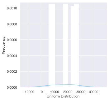
Now we can analyze Probability Distibution below.
# for inline plots in jupyter
%matplotlib inline
# import matplotlib
import matplotlib.pyplot as plt
# for latex equations
from IPython.display import Math, Latex
# for displaying images
from IPython.core.display import Image
# import seaborn
import seaborn as sns
# settings for seaborn plotting style
sns.set(color_codes=True)
# settings for seaborn plot sizes
sns.set(rc={'figure.figsize':(5,5)})
# Write your function below

# Graded-Funtion Begin
ax = sns.distplot(df1,
                  bins=100,
                  kde=True,
                  color='skyblue',
                  hist_kws={"linewidth": 15,'alpha':1})
ax.set(xlabel='Uniform Distribution ', ylabel='Frequency')


# Graded-Funtion End
[Text(0, 0.5, 'Frequency'), Text(0.5, 0, 'Uniform Distribution ')]
Now we can analyze Confidence Intervals below.
df.head()
| BOROUGH | NEIGHBORHOOD | BUILDING CLASS CATEGORY | TAX CLASS AT PRESENT | BLOCK | LOT | BUILDING CLASS AT PRESENT | ADDRESS | APARTMENT NUMBER | ZIP CODE | RESIDENTIAL UNITS | COMMERCIAL UNITS | TOTAL UNITS | LAND SQUARE FEET | GROSS SQUARE FEET | YEAR BUILT | TAX CLASS AT TIME OF SALE | BUILDING CLASS AT TIME OF SALE | SALE PRICE | SALE DATE | |
|---|---|---|---|---|---|---|---|---|---|---|---|---|---|---|---|---|---|---|---|---|
| 0 | 1 | ALPHABET CITY | 07 RENTALS - WALKUP APARTMENTS | 2A | 392 | 6 | C2 | 153 AVENUE B | 10009 | 5 | 0 | 5 | 1633.0 | 6440.0 | 1900 | 2 | C2 | 6625000.0 | 2017-07-19 | |
| 1 | 1 | ALPHABET CITY | 07 RENTALS - WALKUP APARTMENTS | 2 | 399 | 26 | C7 | 234 EAST 4TH STREET | 10009 | 28 | 3 | 31 | 4616.0 | 18690.0 | 1900 | 2 | C7 | NaN | 2016-12-14 | |
| 2 | 1 | ALPHABET CITY | 07 RENTALS - WALKUP APARTMENTS | 2 | 399 | 39 | C7 | 197 EAST 3RD STREET | 10009 | 16 | 1 | 17 | 2212.0 | 7803.0 | 1900 | 2 | C7 | NaN | 2016-12-09 | |
| 3 | 1 | ALPHABET CITY | 07 RENTALS - WALKUP APARTMENTS | 2B | 402 | 21 | C4 | 154 EAST 7TH STREET | 10009 | 10 | 0 | 10 | 2272.0 | 6794.0 | 1913 | 2 | C4 | 3936272.0 | 2016-09-23 | |
| 4 | 1 | ALPHABET CITY | 07 RENTALS - WALKUP APARTMENTS | 2A | 404 | 55 | C2 | 301 EAST 10TH STREET | 10009 | 6 | 0 | 6 | 2369.0 | 4615.0 | 1900 | 2 | C2 | 8000000.0 | 2016-11-17 |
# Write your function below
dx = df[["SALE PRICE", "BOROUGH"]].dropna()
# dx
pd.crosstab(dx['SALE PRICE'], dx['BOROUGH'])
# Graded-Funtion Begin
| BOROUGH | 1 | 2 | 3 | 4 | 5 |
|---|---|---|---|---|---|
| SALE PRICE | |||||
| 0.000000e+00 | 0 | 1826 | 8186 | 0 | 0 |
| 1.000000e+00 | 30 | 22 | 37 | 28 | 9 |
| 2.000000e+00 | 2 | 0 | 0 | 1 | 0 |
| 3.000000e+00 | 0 | 1 | 0 | 1 | 0 |
| 5.000000e+00 | 0 | 0 | 1 | 0 | 0 |
| ... | ... | ... | ... | ... | ... |
| 5.650000e+08 | 1 | 0 | 0 | 0 | 0 |
| 6.200000e+08 | 1 | 0 | 0 | 0 | 0 |
| 6.520000e+08 | 1 | 0 | 0 | 0 | 0 |
| 1.040000e+09 | 1 | 0 | 0 | 0 | 0 |
| 2.210000e+09 | 1 | 0 | 0 | 0 | 0 |
10007 rows × 5 columns
p_fm = 1826/(1826+22)
p_fm
0.9880952380952381
n = 1826+22
n
1848
br_2 = np.sqrt(p_fm * (1 - p_fm) / n)
br_2
0.002522950772404102
z_score = 1.96
lcb = p_fm - z_score* br_2 #lower limit of the CI
ucb = p_fm + z_score* br_2 #upper limit of the CI
print('Confidence interval ',lcb, ucb)
Confidence interval 0.9831502545813261 0.9930402216091502
Make your Hypothesis Testing below
import statsmodels.api as sm
import numpy as np
import matplotlib.pyplot as plt
import pandas as pd
df
| BOROUGH | NEIGHBORHOOD | BUILDING CLASS CATEGORY | TAX CLASS AT PRESENT | BLOCK | LOT | BUILDING CLASS AT PRESENT | ADDRESS | APARTMENT NUMBER | ZIP CODE | RESIDENTIAL UNITS | COMMERCIAL UNITS | TOTAL UNITS | LAND SQUARE FEET | GROSS SQUARE FEET | YEAR BUILT | TAX CLASS AT TIME OF SALE | BUILDING CLASS AT TIME OF SALE | SALE PRICE | SALE DATE | |
|---|---|---|---|---|---|---|---|---|---|---|---|---|---|---|---|---|---|---|---|---|
| 0 | 1 | ALPHABET CITY | 07 RENTALS - WALKUP APARTMENTS | 2A | 392 | 6 | C2 | 153 AVENUE B | 10009 | 5 | 0 | 5 | 1633.0 | 6440.0 | 1900 | 2 | C2 | 6625000.0 | 2017-07-19 | |
| 1 | 1 | ALPHABET CITY | 07 RENTALS - WALKUP APARTMENTS | 2 | 399 | 26 | C7 | 234 EAST 4TH STREET | 10009 | 28 | 3 | 31 | 4616.0 | 18690.0 | 1900 | 2 | C7 | NaN | 2016-12-14 | |
| 2 | 1 | ALPHABET CITY | 07 RENTALS - WALKUP APARTMENTS | 2 | 399 | 39 | C7 | 197 EAST 3RD STREET | 10009 | 16 | 1 | 17 | 2212.0 | 7803.0 | 1900 | 2 | C7 | NaN | 2016-12-09 | |
| 3 | 1 | ALPHABET CITY | 07 RENTALS - WALKUP APARTMENTS | 2B | 402 | 21 | C4 | 154 EAST 7TH STREET | 10009 | 10 | 0 | 10 | 2272.0 | 6794.0 | 1913 | 2 | C4 | 3936272.0 | 2016-09-23 | |
| 4 | 1 | ALPHABET CITY | 07 RENTALS - WALKUP APARTMENTS | 2A | 404 | 55 | C2 | 301 EAST 10TH STREET | 10009 | 6 | 0 | 6 | 2369.0 | 4615.0 | 1900 | 2 | C2 | 8000000.0 | 2016-11-17 | |
| ... | ... | ... | ... | ... | ... | ... | ... | ... | ... | ... | ... | ... | ... | ... | ... | ... | ... | ... | ... | ... |
| 84543 | 5 | WOODROW | 02 TWO FAMILY DWELLINGS | 1 | 7349 | 34 | B9 | 37 QUAIL LANE | 10309 | 2 | 0 | 2 | 2400.0 | 2575.0 | 1998 | 1 | B9 | 450000.0 | 2016-11-28 | |
| 84544 | 5 | WOODROW | 02 TWO FAMILY DWELLINGS | 1 | 7349 | 78 | B9 | 32 PHEASANT LANE | 10309 | 2 | 0 | 2 | 2498.0 | 2377.0 | 1998 | 1 | B9 | 550000.0 | 2017-04-21 | |
| 84545 | 5 | WOODROW | 02 TWO FAMILY DWELLINGS | 1 | 7351 | 60 | B2 | 49 PITNEY AVENUE | 10309 | 2 | 0 | 2 | 4000.0 | 1496.0 | 1925 | 1 | B2 | 460000.0 | 2017-07-05 | |
| 84546 | 5 | WOODROW | 22 STORE BUILDINGS | 4 | 7100 | 28 | K6 | 2730 ARTHUR KILL ROAD | 10309 | 0 | 7 | 7 | 208033.0 | 64117.0 | 2001 | 4 | K6 | 11693337.0 | 2016-12-21 | |
| 84547 | 5 | WOODROW | 35 INDOOR PUBLIC AND CULTURAL FACILITIES | 4 | 7105 | 679 | P9 | 155 CLAY PIT ROAD | 10309 | 0 | 1 | 1 | 10796.0 | 2400.0 | 2006 | 4 | P9 | 69300.0 | 2016-10-27 |
83783 rows × 20 columns
Null Hypothesis: sale price BOROUGH1>BOROUGH2
Alternative Hypthosis: sale price BOROUGH1<BOROUGH2
# Write your function below
b1 = df[df['BOROUGH'] == 1]
b2 = df[df['BOROUGH'] == 2]

# Graded-Funtion Begin
n1 = len(b1)
mu1 = b1["SALE PRICE"].mean()
sd1 = b1["SALE PRICE"].std()

n2 = len(b2)
mu2 = b2["SALE PRICE"].mean()
sd2 = b2["SALE PRICE"].std()

print(n1, mu1, sd1)
print(n2, mu2, sd2)


# Graded-Funtion End
18102 3344641.9823292056 24140481.087110177
6994 594677.118387189 2793509.0485762
sm.stats.ztest(b1["SALE PRICE"].dropna(), b2["SALE PRICE"].dropna(),alternative='two-sided')
(9.495736658776908, 2.1865980196322893e-21)
Write your final conclusion below.
because of p-value b2 smaller than b1, then null hypothesis is correct \